Hierarchical Time Series Data
Many real-world time series data assert some internal structure among the series. For example, the dataset used in the M5 competition is the sales data of different items but with the store and category information provided1. For simplicity, we simplified the dataset to only include the hierarchy of stores.
The simplified dataset can be found here. The original data can be found on the website of IIF. In this simplified version of the M5 dataset, we have the following hierarchy.
flowchart LR

top["Total Sales"]

ca["Sales in California"]
tx["Sales in Texas"]
wi["Sales in Wisconsin"]

top --- ca
top --- tx
top --- wi

subgraph California
ca1["Sales in Store #1 in CA"]
ca2["Sales in Store #2 in CA"]
ca3["Sales in Store #3 in CA"]
ca4["Sales in Store #4 in CA"]

ca --- ca1
ca --- ca2
ca --- ca3
ca --- ca4
end


subgraph Texas
tx1["Sales in Store #1 in TX"]
tx2["Sales in Store #2 in TX"]
tx3["Sales in Store #3 in TX"]

tx --- tx1
tx --- tx2
tx --- tx3

end


subgraph Wisconsin
wi1["Sales in Store #1 in WI"]
wi2["Sales in Store #2 in WI"]
wi3["Sales in Store #3 in WI"]

wi --- wi1
wi --- wi2
wi --- wi3

end
The above tree is useful when thinking about the hierarchies. For example, it explicitly tells us that the sales in stores #1, #2, #3 in TX should sum up to the sales in TX.
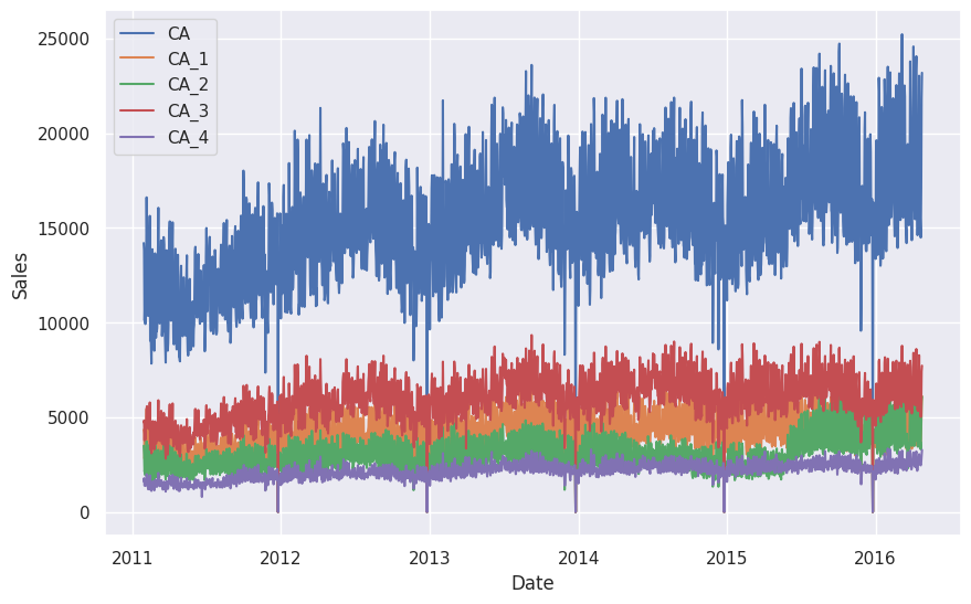
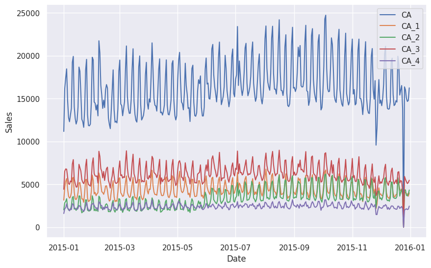
We plotted the sales in CA as well as the individual stores in CA. We can already observe some synchronized anomalies.
Summing Matrix
The relations between the series is represented using a summing matrix \(\mathbf S\), which connects the bottom level series \(\mathbf b\) and all the possible levels \(\mathbf s\)2
If our forecasts satisfy this relation, we claim our forecasts to be coherent2.
Summing Matrix Example
We take part of the above dataset and only consider the hierarchy of states,
The hierarchy is also revealed in the following tree.
flowchart TD

top["Total Sales"]

ca["Sales in California"]
tx["Sales in Texas"]
wi["Sales in Wisconsin"]

top --- ca
top --- tx
top --- wi
In this example, the bottom level series are denoted as
and all the possible levels are denoted as
The summing matrix is
-
Makridakis S, Spiliotis E, Assimakopoulos V. The M5 competition: Background, organization, and implementation. Int J Forecast. 2022;38: 1325–1336. doi:10.1016/j.ijforecast.2021.07.007 ↩
-
Hyndman, R.J., & Athanasopoulos, G. (2021) Forecasting: principles and practice, 3rd edition, OTexts: Melbourne, Australia. OTexts.com/fpp3. Accessed on 2022-11-27. ↩↩