Time Series Data Generating Process: Langevin Equation
Among the many data generating processes (DGP), the Langevin equation is one of the most interesting DGP.
Brownian Motion
Brownian motion as a very simple stochastic process can be described by the Langevin equation1. In this section, we simulate a time series dataset from Brownian motion.
Macroscopically, Brownian Motion can be described by the notion of random forces on the particles,
where \(v(t)\) is the velocity at time \(t\) and \(R(t)\) is the stochastic force density from the reservoir particles. Solving the equation, we get
To generate a dataset numerically, we discretize it by replacing the integral with a sum,
where \(t_i = i * \Delta t\) and \(t = t_n\), thus the equation is further simplified,
The first term in the solution is responsible for the exponential decay and the second term calculates the effect of the stochastic force.
To simulate a Brownian motion, we can either use the formal solution or the differential equation itself. Here we choose to use the differential equation itself. To simulate the process numerically, we rewrite
as
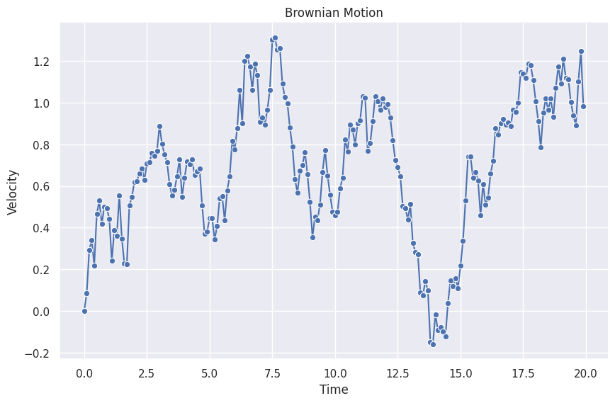
The following is a simulated 1D Brownian motion.
We create a stepper to calculate the next steps.
import numpy as np
import copy
import matplotlib.pyplot as plt
import seaborn as sns; sns.set()

## Define Brownian Motion
class GaussianForce:
"""A Gaussian stochastic force iterator.
Each iteration returns a single sample from the corresponding
Gaussian distribution.

:param mu: mean of the Gaussian distribution
:param std: standard deviation of the Gaussian distribution
:param seed: seed for the random generator
"""

def __init__(self, mu: float, std: float, seed: Optional[float] = None):
    self.mu = mu
    self.std = std
    self.rng = np.random.default_rng(seed=seed)

def __next__(self) -> float:
    return self.rng.normal(self.mu, self.std)


class BrownianMotionStepper:
    """Calculates the next step in a brownian motion.

    :param gamma: the damping factor $\gamma$ of the Brownian motion.
    :param delta_t: the minimum time step $\Delta t$.
    :param force_densities: the stochastic force densities, e.g. [`GaussianForce`][eerily.data.generators.brownian.GaussianForce].
    :param initial_state: the initial velocity $v(0)$.
    """

    def __init__(
        self,
        gamma: float,
        delta_t: float,
        force_densities: Iterator,
        initial_state: Dict[str, float],
    ):
        self.gamma = gamma
        self.delta_t = delta_t
        self.forece_densities = copy.deepcopy(force_densities)
        self.current_state = copy.deepcopy(initial_state)

    def __iter__(self):
        return self

    def __next__(self) -> Dict[str, float]:

        force_density = next(self.forece_densities)
        v_current = self.current_state["v"]

        v_next = v_current + force_density * self.delta_t - self.gamma * v_current * self.delta_t

        self.current_state["force_density"] = force_density
        self.current_state["v"] = v_next

        return copy.deepcopy(self.current_state)

## Generating time series
delta_t = 0.1
stepper = BrownianMotionStepper(
    gamma=0,
    delta_t=delta_t,
    force_densities=GaussianForece(mu=0, std=1),
    initial_state={"v": 0},
)

length = 200

history = []
for _ in range(length):
    history.append(next(stepper))

df = pd.DataFrame(history)

fig, ax = plt.subplots(figsize=(10, 6.18))
sns.lineplot(
    x=np.linspace(0, length-1, length) * delta_t,
    y=df.v,
    ax=ax,
    marker="o",
)

ax.set_title("Brownian Motion")
ax.set_xlabel("Time")
ax.set_ylabel("Velocity")
-
Ma L. Brownian Motion — Statistical Physics Notes. In: Statistical Physics [Internet]. [cited 17 Nov 2022]. Available: https://statisticalphysics.leima.is/nonequilibrium/brownian-motion.html ↩