Generating Processes for Time Series
The data generating processes (DGP) for time series are diverse. For example, in physics, we have all sort of dynamical systems that generates time series data and many dynamics models are formulated based on the time series data. In industries, time series data are often coming from stochastic processes.
We present some data generating processes to help us build up intuition when modeling real-world data.
Simple Examples of DGP
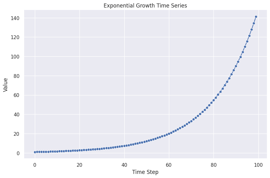
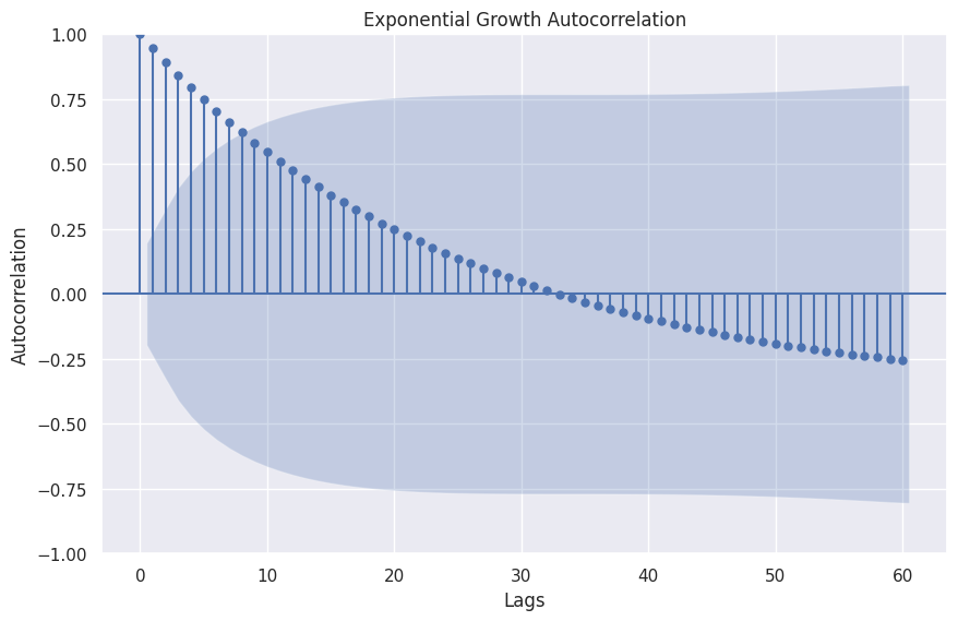
Exponential Growth
Exponential growth is a frequently observed natural and economical phenomenon.
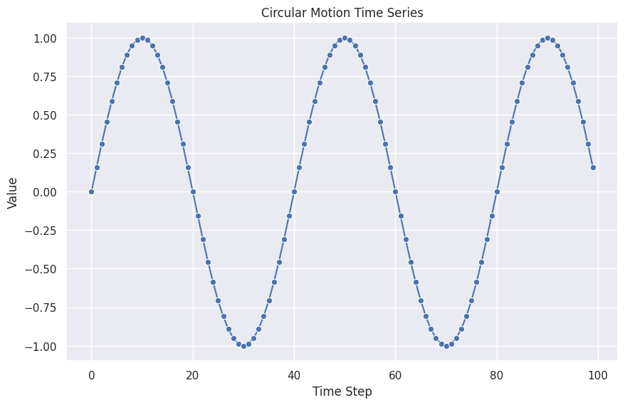
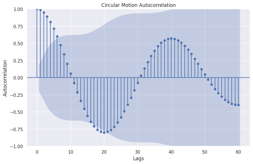
Circular Motion
The circular motion shows some cyclic patterns.
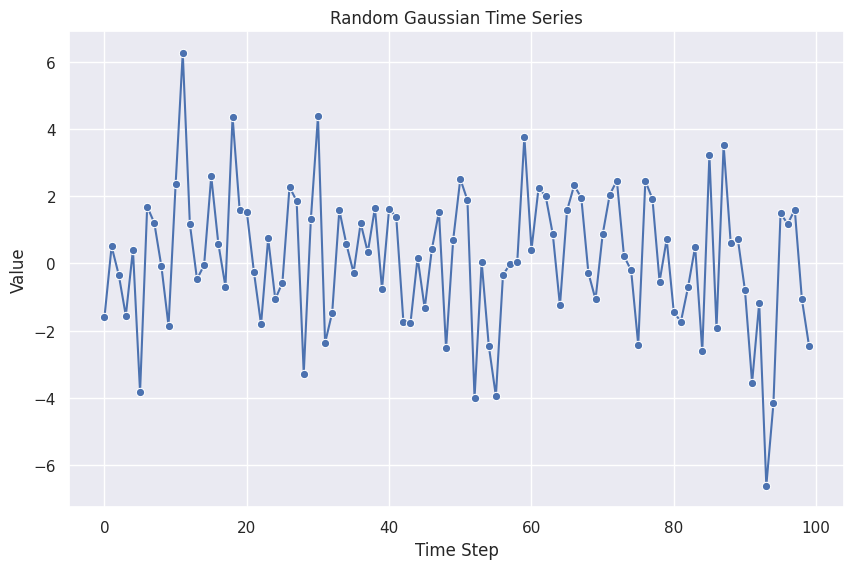
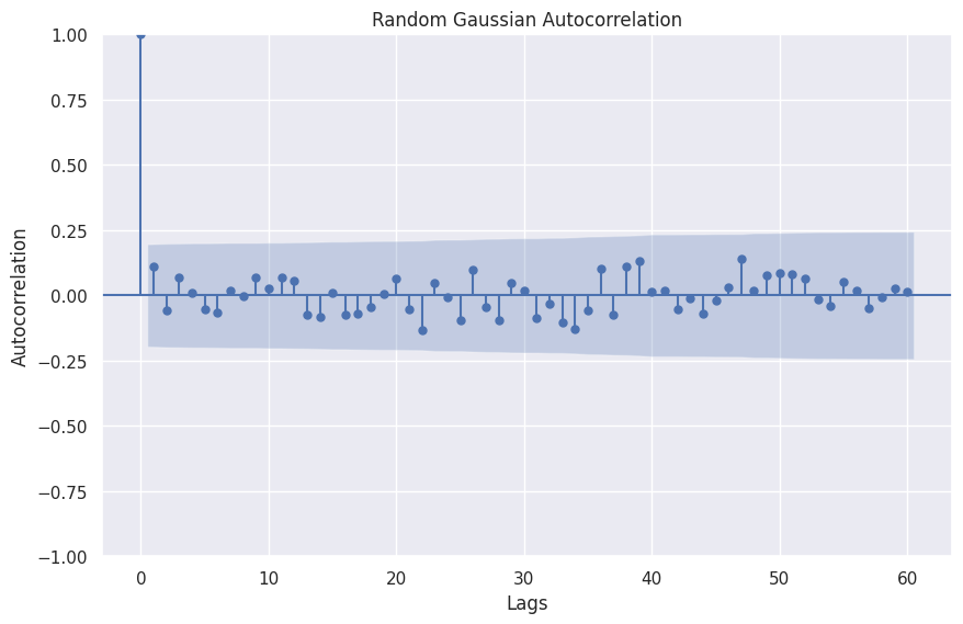
Random Gaussian
Time series can also be noisy Gaussian samples.
General Linear Processes
A popular model for modeling as well as generating time series is the autoregressive (AR) model. An AR is formulated as
AR(p) and the Lag Operator
A general autoregressive model of p-th order is
where \(l\) is the lag.
Define a lag operator \(\hat L\) with \(\hat L x_t = x_{t-1}\). The definition can also be rewritten using the lag operator
We write down each time step in the following table.
| \(t\) | \(x_t\) |
|---|---|
| 0 | \(y_0\) |
| 1 | \(\phi_0 + \phi_1 y_0 + \epsilon_1\) |
| 2 | \(\phi_0 + \phi_1 (\phi_0 + \phi_1 y_0 + \epsilon_1) + \epsilon_2 = \phi_0 (1 + \phi_1) + \phi_1^2 y_0 + \phi_1\epsilon_1 + \epsilon_2\) |
| 3 | \(\phi_0 + \phi_1 (\phi_0 + \phi_1\phi_0 + \phi_1^2 y_0 + \phi_1\epsilon_1 + \epsilon_2) + \epsilon_3 = \phi_0(1 + \phi_1 + \phi_1^2) + \phi_1^3 y_0 + \phi_1^2\epsilon_1 + \phi_1\epsilon_2 + \epsilon_3\) |
| ... | ... |
| \(t\) | \(\phi_0 \sum_{i=0}^{t-1} \phi_1^i + \phi_1^t y_0 + \sum_{i=1}^{t-1} \phi_1^{t-i} \epsilon_{i}\) |
We have found a new formula for AR(1), i.e.
which is very similar to a general linear process1
The general linear process is the Taylor expansion of an arbitrary DGP \(x_t = \operatorname{DGP}(\epsilon_t, ...)\)1.
Interactions between Series
The interactions between the series can be modeled as explicit interactions, e.g., many spiking neurons, or through hidden variables, e.g., hidden state model2. Among these models, Vector Autoregressive model, aka VAR, is a simple but popular model.
-
Das P. Econometrics in Theory and Practice. Springer Nature Singapore; doi:10.1007/978-981-32-9019-8 ↩↩
-
Contributors to Wikimedia projects. Hidden Markov model. In: Wikipedia [Internet]. 22 Oct 2022 [cited 22 Nov 2022]. Available: https://en.wikipedia.org/wiki/Hidden_Markov_model ↩